Neural network is a modern machine learning method that has been widely adopted. However, random forest, an improvement of the traditional decision tree may be a better choice for some problems because of its simplicity and much lower computational cost.

A random forest is an ensemble of decision trees that have a different set of random features both in features and number of features, with varying depths in a forest of a given number of trees.

We start with a video lecture evaluation problem. Based on the features of the lecture to draw conclusions whether students are interested in the lecture or not.

The dataset is data.csv file. There are six features that are six columns of input data:

title_word_count – number of words in the title of the lecture.

document_entropy – variety of topics.

easiness – easiness of text. A lower score corresponds to a more difficult representation language.

fraction_stopword_presence – the fraction of stopwords such as “the” or “and” that appear in the lecture.

speaker_speed – the average speaking rate in words per minute of the presenter in the video.

silent_period_rate – the fraction of time in the lecture video that is silence.

The resulting data column is ‘engagement’ – True if the learner watches the video attentively, False otherwise.

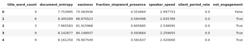
We read the data file and display the first 5 rows

import pandas as pd
import numpy as np
from sklearn.model_selection import train_test_split, GridSearchCV
from sklearn.ensemble import RandomForestClassifier
from sklearn.metrics import precision_score

df = pd.read_csv('data.csv')
to_keep = ['title_word_count', 'document_entropy', 'easiness', 'fraction_stopword_presence',
               'speaker_speed', 'silent_period_rate', 'engagement']
df = df[to_keep]
df.head()

Notice the ‘engagement’ column. It seems that most of the students skip the lectures

np.mean(df['engagement'])
0.09708842948371035

Thus, only about 10% of watching the video thoroughly. This is an unbalanced binary classification problem where positive numbers are in the minority. Restate the problem with the result reversed, the positive number becoming the majority will give a more accurate result. Rename the ‘engagement’ column to ‘not_engagement’

df = df.rename({'engagement': 'not_engagement'}, axis = 1)
df['not_engagement'] = -df['not_engagement']
df.head()

We perform train-test split:

df_X = df.iloc[:, :-1]
df_y = df.iloc[:, -1]
X_train, X_test, y_train, y_test = train_test_split(df_X, df_y, random_state = 0)

We are comparing two models random forest and neural network. They need to be reliably evaluated, so cross-validation is required. The construction of the model grid satisfies both cross-validation and parameter optimization. There are three parameters for the random forest:

n_estimators – number of trees in the forest.

max_depth – small depth reduces complexity and overfitting.

max_features – small max_features increases generalization and reduces overfitting.

In this problem we want to look at the less interesting lectures to learn from, so positive precision is needed. Metric for evaluation is ‘precision’

params_grid_rf = {'n_estimators': [30, 40, 50, 60], 'max_depth': [10, 20, 30], 'max_features': [3, 4, 5]}
grid_rf = RandomForestClassifier(random_state = 0, n_jobs = 20)
grid_rf = GridSearchCV(grid_rf, param_grid = params_grid_rf, scoring = 'precision')
grid_rf.fit(X_train, y_train)

The validation score is:

grid_rf.best_score_
0.9448751118818786

Optimal parameters:

grid_rf.best_params_
{'max_depth': 20, 'max_features': 4, 'n_estimators': 50}

The optimal forest has 50 trees with a maximum depth of 20 and a maximum number of features of 4 (4 out of 6 features).

Now we optimize the neural network with the following parameters:

hidden_layer_sizes – number of hidden nodes

alpha – penalty coefficient (L2 regularization)

solver – weight optimization method

activation – activation function or transfer function

tol – optimization tolerance. When the validation score does not improve by at least a tol amount for every generation for 10 consecutive generations, the network is considered convergent and training stops if early_stopping is set to True.

early_stopping – stop training early to reduce computation cost and prevent overfitting

Construct grid parameters:

params_grid_nn = {'hidden_layer_sizes': [30, 40, 50],
               'alpha': [0.0001, 0.001],
               'solver': ['lbfgs', 'adam'],
               'activation': ['logistic', 'relu'],
               'tol': [0.0001, 0.0002],
               'early_stopping': [True, False]
              }

While random forests can use feature data directly, feature normalization is a requirement for neural networks

from sklearn.neural_network import MLPClassifier
from sklearn.preprocessing import MinMaxScaler

scaler = MinMaxScaler()

X_train_scaled = scaler.fit_transform(X_train)
X_test_scaled = scaler.transform(X_test)

Network training:

grid_nn = MLPClassifier(random_state = 0, max_iter = 10000)
grid_nn = GridSearchCV(grid_nn, param_grid = params_grid_nn, scoring = 'precision')
grid_nn.fit(X_train_scaled, y_train)

The validation score:

grid_nn.best_score_
0.9453020149599608

Optimal parameters:

grid_nn.best_params_
{'activation': 'logistic',
 'alpha': 0.0001,
 'early_stopping': True,
 'hidden_layer_sizes': 40,
 'solver': 'lbfgs',
 'tol': 0.0001}

To sum up, the validation score of the random forest is 0.9448751118818786, and the validation score of the neural network is 0.9453020149599608. The neural network has shown strength, it scores higher. The random forest has a lower but insignificant score and with much lower computational cost and simplicity in installation, it is a better choice for the classification model.

Once the random forest model has been selected, we build the model with the optimal parameters:

model = RandomForestClassifier(random_state = 0, n_jobs = 20,
                               max_depth=20,
                               max_features=4,
                               n_estimators=50
                              ).fit(X_train, y_train)

Evaluate the model with the test set for the validated optimal model, with the metric being ‘precision’:

pred = model.predict(X_test)
precision_score(y_test, pred)
0.9419622293873791

Using the model:

input = np.array([8, 10.15, 60.1, 0.7, 4.1, 0.1]).reshape(-1,6)
input = pd.DataFrame(input, columns = to_keep[:-1])
model.predict(input)

The result is:

array([ True])